[Sheet music] Murder, she wrote piano theme - La signora in giallo

Scarica lo spartito/Download sheet music.

How to contact Facebook or delete your account

Contacting Facebook can really be a pain, but definitely deleting your account is even harder. Since they rely on your data to survive, they will hang on to it as long as possible.

Luckily, Mary Smith gathered all possible ways to contact Facebook and receive support. Feature requests, suggestions, bug reports and account deletion can all be found there.

You can even request Facebook to send you a CD copy of all the data they have about you accordingly with your country's privacy laws.

By the way, good luck at getting Facebook to reply to you, especially with the data request. If they don't answer, insist since they MUST satisfy your request within a limited time.

UPDATE: An anonymous user pointed out that more information about that is available at  webmarketing-conseil.

Legend of Dragoon fix disc 2 freeze after Lenus & Regole battle

ENGLISH: please refer to supercheats, quick summary: beat the battle without ever going Dragoon

ITALIANO:

The Legend of Dragoon é uno di quei giochi che non risentono dell’etá. Purtroppo, se si prova a giocarlo su una qualsiasi console che non sia la ormai rara PlayStation 1 (PS2, PS3, PSP o usando  l’emulatore PSX), per qualche motivo dopo la battaglia contro Lenus e Regole verso la fine del disco 2, lo schermo diventa nero ed il gioco va in freeze senza possibilitá di recupero.

GNOME 3 add applications taskbar/panel

GNOME 3 does not have, like GNOME 2, two taskbars: one for the applications and one for the system tray. It is possible to add the application taskbar (which includes a system tray panel too) manually with the project tint2. All instructions for installing under different distros are available directly on the developers website.

ITALIANO:

GNOME 3 enable right click on desktop and show icons

GNOME 3 by default doen’t show any icon on the desktop and does not allow right-clicking it. You could change this behaviour manually:

• run yum install dconf-editor as root or install it via add/remove software and launch it when it’s ready
• navigate the menus through org –> GNOME –> Desktop –> Background
• search for the show-desktop-icons entry and chek its checkbox

ITALIANO:

GNOME 3 add minimize and restore buttons to windows

GNOME 3 by default shows only the “close” button on windows. You could add the other two (minimize and restore/maximize) manually:

• run yum install gconf-editor as root or install it via add/remove software and launch it when it’s ready
• navigate the menus through Desktop –> GNOME –> Shell –> Windows
• search for the button_layout entry and edit its value to :minimize,maximize,close (colon included!)
• restart nautilus or log out and in again to see the changes take effect

ITALIANO:

Realtek wireless on Fedora

This article applies to the 819x Realtek wireless cards series like models 8191SEvB, 8191SEvA2, 8192SE, …

Main reference site is Stanislaw Gruszka’s compact wireless website.

You can either try the -stable version or the –next. Both have different kernel requirements, the –next version, though more unstable, is compiled against the latest kernel version so you should run yum update kernel as root before installing the appropriate package for your system.

After installation you will have to reboot the system before being able to use and control your wireless card through NetworkManager.

 

ITALIANO:

 

Questo articolo si applica ai modelli di schede wireless Realtek serie 819x quali 8191SEvB, 8191SEvA2, 8192SE, …

Il sito di riferimento é compact wireless di Stanislaw Gruszka.

Potete provare sia la versione -stable che la –next. Entrambe hanno differenti requisiti di kernel, la versione –next, sebbene piú instabile, é compilata per l’ultima versione del kernel supportata dal sistema per cui é sufficiente lanciare yum update kernel da root prima di installare il pacchetto corretto per il proprio sistema.

Al termine dell’installazione sará necessario riavviare il sistema prima di poter usare e controllare la propria scheda wireless attraverso il NetworkManager.

[MatLab] EM – Expectation Maximization reconstruction technique implementation

EM – Expectation Maximization is an iterative algorithm used in tomographic images (as in CT) reconstruction, very useful when the FBP – Filtered Back Projection technique is not applicable.

Basic formula is:

f_k+1 = (f_k / alpha) (At (g / (A f_k)))

where:

• f_k is solution (the resulting reconstructed image) at k-th iteration, at first iteration it is our guess
• g is image sinogram (what we get from the scanning)
• A f_k is Radon transform of f_k
• At is inverse Radon
• alpha is inverse Radon of a sinogram with all values 1 which represents our scanning machine

%EM - Expectation Maximization
%Formula is:
%f_k+1 = (f_k / alpha) (At (g / (A f_k)))
%f_k is solution at k-th iteration, at first iteration it is our guess
%g is image sinogram
%A f_k is Radon transform of f_k
%At is inverse Radon of its argument
%alpha is inverse Radon of a sinogram with all values 1 which represents our scanning machine

%clear matlab environment
clear all;
close all;
theta=[0:89]; %limited projection angle 90 degrees instead of 180
F=phantom(64); %create test phantom 64x64 pixels aka alien
figure, imshow(F,[]),title('Alien vs Predator'); %show alien
S1 = sum(sum(F));%calculate pixels sum on F
R = radon(F,theta); %apply Radon aka scan the alien to create a sinogram
figure, imshow(R,[]),title('Sinoalien');%show sinogram
%set all values <0 to 0
index=R<0;
R(index)=0;
n = 2000;%iterations
Fk=ones(64);%our initial guess
%create alpha aka pixels sum of the projection matrix (our scanning machine)
sinogramma1=ones(95,90);
alpha=iradon(sinogramma1, theta,'linear', 'none', 1,64);
%calculate relative error
relerrfact=sum(sum(F.^2));
for  k=1:n
     Afk = radon(Fk,theta);%create sinogram from current step solution
     %calculate g / A f_k=Noised./(A f_k+eps); aka initial sinogram / current step sinogram
     %eps is matlab thing to prevent 0 division
     GsuAFK=R./(Afk+eps);
     retro=iradon(GsuAFK, theta, 'linear', 'none', 1,64);%At (g / (A f_k))
     %multiply current step with previous step result and divide for alpha updating f_k
     ratio=Fk./alpha;
     Fk=ratio.*retro;
     %normalize
     St = sum(sum(Fk));
     Fk = (Fk/St)*S1;
	 %calculate step improvement
     Arrerr(k) = sum(sum((F - Fk).^2))/relerrfact;
	 %stop when there is no more improvement
     if((k>2) &&(Arrerr(k)>Arrerr(k-1)))
        break;
     end     
end
figure, imshow(Fk,[]),title('Fk');%show reconstructed alien
figure, plot(Arrerr),title('Arrerr');%show error improvement over all iterations

%compare our result with the one we would have had using the FBP - Filtered Back Projection
easy=iradon(R,theta, 'Shepp-Logan',1,64);
figure, imshow(easy,[]),title('FBP');

%calculate error between EM and FBP - with limited image size and projection degree FBP is bad!
FBPerr=sum(sum((F - easy).^2))/relerrfact;

[MatLab] SIRT - Simultaneous Iterative Reconstruction Technique implementation

SIRT – Simultaneous (algebraic) Reconstruction Technique is an iterative algorithm used in tomographic images (as in CT) reconstruction, very useful when the FBP – Filtered Back Projection technique is not applicable.

Basic formula is:

f_(k+1) = f_k + At (g - A f_K)

where:

• f_k is solution (the resulting reconstructed image) at k-th iteration, at first iteration it is our guess
• g is image sinogram (what we get from the scanning)
• A f_k is Radon transform of f_k
• At is inverse Radon

Note: this sample code is to showcase the algorithm. It does not use FBP for the iradon, it adds noise, it normalizes the image values as per OUR needs. Given these difficult conditions, it still produces an amazing result.

Please check the comments carefully and tailor it to your use case!

    

%SIRT - Simultaneous Iterative Reconstruction Technique
%Formula is:
%f_(k+1) = f_k + At (g - A f_K)
%f_k is solution at k-th iteration, at first iteration it is our guess
%g is image sinogram
%A f_k is Radon transform of f_k
%At is inverse Radon of its argument

%This example shows how to scan an image with a limited angle, obtain the sinogram, add noise to make things worse, and reconstruct the initial image with great accuracy
%You may want to remove/edit some sections if you intend to apply this to your use case:
%- skip/correct normalization
%- skip noise
%- use FBP for the iradon

%clear matlab environment
clear all;
close all;
theta = [0:179]; %projection angle 180 degrees
F = phantom(128); %create new test phantom 128x128 pixels aka alien. You can use your own image here if you want. It was not tested on non-grayscale images
figure, imshow(F,[]),title('Alien vs Predator'); %show alien
S1 = sum(sum(F));%calculate pixels sum on F
R = radon(F,theta);%apply Radon aka scan the alien to create a sinogram
figure, imshow(R,[]),title('Sinoalien');%show sinogram
%add image noise to the sinogram. You can skip this part, it's just to showcase the algorithm, it's not obviously needed
maximum=max(max(R));
minimum=min(min(R));
R=(R-minimum)/(maximum-minimum);
%normalize between 0 and 1. You can tune this as per your needs
fact=1001;%set the number of X-rays, the higher the better (and deadlier)
R=(fact/10^12)*R;
Noised=imnoise(R,'poisson');%add Poissonian noise
figure, imshow(Noised,[]),title('Dirty alien');%show noisy sinogram
%This part below you actually need it! Edit accordingly to your case
%At applied to g aka noisy alien
%Check the parameters here if you edited the code above! You might also want to tune the parameters for the iradon. Here we're showing that this works even when the FBP is not available!
At = iradon(Noised,theta,'linear', 'none', 1,128); %reconstruct noisy alien.
figure, imshow(At,[]),title('At G'); %show noisy alien
%algorithm starts crunching here
S2 = sum(sum(At)); %calculate pixels sum on At
At = (At/S2)*S1; %normalize At so that pixel counts match. Edit as per your needs
n = 100;%iterations. Might be more, there's always a limit over which it doesn't make sense to keep iterating though!
Fk = At;%Matrix Fk is our solution at the k-th step, now it is our initial guess
for  k=1:n
    t = iradon(radon(Fk,theta),theta, 'linear', 'none', 1,128);% reconstruct alien using Fk unfiltered sinogram. Maybe use FBP if you want here
    %normalize. Again, as per your needs
    St = sum(sum(t));
    t = (t/St)*S1;
    %update using (At g - At A f_k) 
    %new Fk = Fk + difference between reconstructed aliens At_starting - t_previuous_step
    Fk = Fk + At - t;
	%remember that our alien is normalized between 0 and 1. Might not be your case!
    %delete values <0 aka not real! Might not be your case!
    index = Fk<0;
    Fk(index)=0;
    %delete values >1 aka not real! Might not be your case!
    index = find(Fk>1);
    Fk(index)=1;
    %show reconstruction progress every 10 steps
    if(mod(k,10)== 0)
    figure,imshow(Fk,[]),title('Fk');
    end
    %calculate step improvement between steps. Tune as per your needs
    Arrerr(k) = sum(sum((F - Fk).^2));
    %stop when there is no more improvement. Tune as per your needs
    if((k>2) &&(Arrerr(k)>Arrerr(k-1)))
       break;
    end
end
figure, plot(Arrerr),title('Arrerr');%show error improvement over all iterations

[MatLab] Filter a tomographic image in Fourier’s space

MatLab has built-in functions to simulate acquisition and elaboration of tomographic (as in CT) images. When it comes to filtering the image prior to back-projecting it, it is possible to do it yourself without relying on the (good as in Shepp-Logan) filters MatLab has.

 

We will filter our image in Fourier’s space. For each column of the sinogram, we:

• apply the Fourier transform
• filter it
• apply the Fourier antitransform

When we reconstruct our image WITHOUT having MatLab apply any filter, we’ll see the image, filtered with our filter, as a result.

%filter an image in Fourier's space

%clear matlab environment
clear all;
close all;
theta = [0:179]; %projection angle 180 degrees
F = phantom(256); %create new test phantom 256x256 pixels aka alien
figure, imshow(F,[]),title('Alien vs Predator'); %show alien
R = radon(F,theta); %apply Radon aka scan the alien to create a sinogram
figure, imshow(R,[]),title('Sinoalien'); %show sinogram
%get Shepp-Logan filter, you can use any filter you want
Fi = phantom(128);
Ri = radon(Fi,theta);
[I, Filter]=iradon(Ri,theta, 'Shepp-Logan');
%add image noise to the sinogram
maximum=max(max(R));
minimum=min(min(R));
R=(R-minimum)/(maximum-minimum);
%normalize between 0 and 1
fact=1001;%set the number of X-rays, the higher the better (and deadlier)
R=(fact/10^12)*R;
Noised=imnoise(R,'poisson');%add Poissonian noise
figure, imshow(Noised,[]),title('Dirty alien');%show noisy sinogram
%add zero-padding
Padded(1:512, 1:180)=0;
Padded(1:367, :) = Noised;
figure, imshow(Padded,[]),title('Padded alien');%show padded sinogram
%filter the noise with our filter in Fourier's space for each column of the sinogram
for k=1:180
	%FPadded = filtered and padded
    FPadded(:, k)=fft(Padded(:, k));%Fourier transform
    FPadded(:, k)=FPadded(:, k).*Filter;%Filter in Fourier
    Padded(:, k)=real(ifft(FPadded(:, k)));%Fourier antitransform of the filtered and still padded sinogram column
end
%remove padding
R=Padded(1:367,:);
figure, imshow(R,[]),title('Unpadded filtered alien');%show final sinogram
I=iradon(R, theta, 'None'); %back project without filtering to show final result
figure, imshow(I,[]),title('Final alien');

[PHP] PageRank implementation

There are two possible PageRank implementations: the power method and the iterative method. We will describe both.

To check the results obtained we provide a scri'pt to generate a .gexf file to be opened with Gephi.

Test datasets are available at the Toronto university website.

Technologies used:

• PHP
• Gephi
• XML
  

1.Power method
 
This method takes longer than the other one, however the result is equally right. Using a sparse matrix instead of the full one may help speed up the process.

Method description:

1. Pick the NxN input matrix and make it stochastic, call it A
2. Create the P" matrix as alpha*A+(1-alpha)*M with alpha a factor which describes the probability of a random jump and M an NxN matrix filled with values 1/N
3. Create starting vector v_0 with length N filled with values 1/N
4. Compute v_m = v_m-1*P" where the first time v_m-1 is exactly v_0
5. Compute the difference v_m - v_m-1 which should converge to 0
6. When the difference doesn't vary over a certain threshold or i iterations have been made, stop. v_m should contain the PageRank for every page

To run the program you must have the nodes and adj_matrix files from the chosen dataset. The implementation source code is found here here.

NOTE: Due to Apache and PHP limitations, you may have to modify the php.ini file to grant more memory to the scripts (if you don't want to store the matrix on filesystem like we did) by setting the memory_limit parameter to at least 768MB and raising the maximum script execution time to 5 minutes(300 seconds) with max_execution_time.

2. Iterative method - found on phpir

To use this method you must have the nodes and adj_list files from the chosen dataset.




Method description:

Each page is given a starting PR of 1/N where N is the number of nodes in the graph. Each page then gives to every page it links a PR of current_page_PR/number_of_outbound_links.
It's introduced a dampening factor alpha (0,15) which represents the probability of making a random jump while visiting the graph or when reaching a cul de sac.

PR_new = alpha/n + (1-alpha)*PR_old



Every PR is then normalized between 0 and 1.

The process keeps going until it has reached i iterations or the difference between old and new PR doesn't vary over a certain threshold.

Our implementation is available here.

3. Gephi parser:

To use the parser you you must have the nodes and adj_list files from the chosen dataset. The parser outputs a .gexf file to be opened with Gephi. Here is a sample .gexf file obtained by parsing the first dataset available on the site (the one about abortion).

pro-AD website: MRI analysis for prodromal Alzheimer’s assessment

Recently I participated in the pro-AD’s website development.

pro-AD is a website created at DIFI, the University of Genoa’s Department of Physics, to help medics automagically analyse MRI images for the prodromal Alzheimer's disease assessment.

Registered medics can easily submit DICOM or NII files through the website to their private local folder via the java applet JUploader or the PHP uploader which is shown automatically when no java plugin is detected on the user's browser. They can then modify the information associated with those images: age, gender and an optional unique ID - no personal data about the patients is stored anywhere anytime during the process.

Easy access for the medic's personal profile is provided through a dedicated page; if a valid e-mail address is provided, it is possible to enable e-mail notifications about processing results.

When one or more files are selected for processing, the server enqueues them in a multithreaded pipeline and starts the analysis. At the end, a single number which describes the patient's likelihood of being affected in the near future by the disease is returned for each file sent to processing. If the file processed was of really bad quality or was not a valid file, the process fails and an error is shown instead of the result.

All results are stored for easy future access and can be viewed and exported in XLS format from a dedicated page. If a file is sent to processing more times, only the latest result is stored.

[PHP] Create XLS document

If you need to create XLS documents via PHP, you may need these functions:

//XLS Begin of file
function xlsBOF() {
echo pack("ssssss", 0x809, 0x8, 0x0, 0x10, 0x0, 0x0);
return;
}
//XLS End of file
function xlsEOF() {
echo pack("ss", 0x0A, 0x00);
return;
}
//Writes a number in a cell
function xlsWriteNumber($Row, $Col, $Value) {
if($Value == null){
xlsWriteLabel($Row, $Col, $Value);
}
else{
echo pack("sssss", 0x203, 14, $Row, $Col, 0x0);
echo pack("d", $Value);
}
return;
}
//Writes a string in a cell
function xlsWriteLabel($Row, $Col, $Value ) {
$L = strlen($Value);
echo pack("ssssss", 0x204, 8 + $L, $Row, $Col, 0x0, $L);
echo $Value;
return;
}

//Creates headers to download the file
function xlsWriteHeader(){
// Send Header
header("Pragma: public");
header("Expires: 0");
header("Cache-Control: must-revalidate, post-check=0, pre-check=0");
header("Content-Type: application/force-download");
header("Content-Type: application/octet-stream");
header("Content-Type: application/download");;
header("Content-Disposition: attachment;filename=EXPORTNAME.xls ");
header("Content-Transfer-Encoding: binary ");
}

[PHP] Send mail with attachment using PEAR

If you use PEAR and want to send mails with attachments via PHP, you may find this helpful.

First, ensure you have installed PEAR’s Mail and Mail_mime packages. Then, you just need a function like this:

 

function send_mail($mail, $subject, $bodytxt, $bodyhtml, $attachment){
    require_once('Mail.php');
    require_once('Mail/mime.php');
    //mail parameters, this is the basic one
    $params = array("host"=>"YOUR_HOST");
    //creates smtp mail object
    $mail_sender = Mail::factory("smtp", $params);
    //creates mail headers
    $headers = array("From"=>"YOUR_ADDRESS", "To"=>$mail, "Subject"=>$subject);
    //creates attachment and body fields
    $crlf = "\n";
    $mime = new Mail_mime($crlf);
    $mime->setTXTBody($bodytxt);
    $mime->setHTMLBody($bodyhtml);
    $mime->addAttachment($attachment, "ATTACHMENT_TYPE");
    //never change these lines order
    $body = $mime->get();
    $headers = $mime->headers($headers);
    $error=$mail_sender->send($mail, $headers, $body);
    return $error;
}

 

where:

• YOUR_HOST is your mail host, something like smtp.gmail.com
• $mail is the recipient’s mail address
• $bodytxt is the mail’s body in TXT format, do not use HTML markup here!
• ATTACHMENT_TYPE is the attachment’s MIME type as per IANA’s specifications, something like image/jpeg
• if you change the order of the last lines, the attach operation will not work

[PHP, XML] Twitter friends graph

Brief example on how to create and draw some Twitter user’s friends graph.

Piccolo esempio di come creare e disegnare il grafo dei friends di un dato utente Twitter.

 

English:

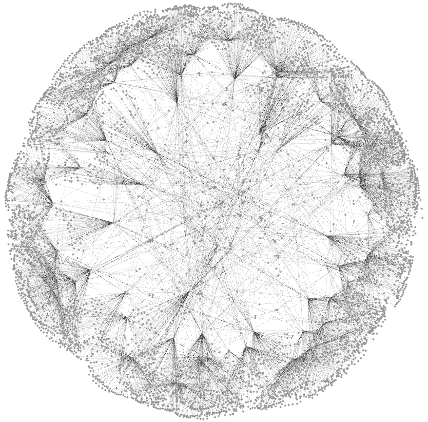
With friends Twitter means “people whom the user follows”. Starting from a chosen user, we grab all his friends until a depth level of 3 and we create a XML file with a proper structure to be opened by Gephi in order to graphically visualize the result. The number of users we get is far lower than the real one due to Twitter API’s limitations.

To create the gexf file for Gephi, just run the HowDoYouGraph script after editing the $username variable with the desired username. After a little coffee break, in the same folder as the script you should find a file named grafo.gexf.

 

Show an example graph for user VivoMikiX and download the gexf source.

 

Stats about the undirected example graph:

• Total nodes: 5013
• Total edges: 5539
• Medium degree = 2.21
• Diameter = 6
• Density = 0
• Modularity = 0.876
  • Number of communities = 72
• Weakly connected components = 1
• Medium clustering coefficient = 0.014
  • Total triangles = 202
• Eigenvector centrality with 300 iterations = 0.0325
• Medium path length = 4.496
  • Number of shortest paths = 25125156
  • Radius = 3

 

Italiano:

Con friends si intendono tutte le persone che l'utente segue. Partendo da un dato utente, recuperiamo i suoi friends fino al livello 3 e generiamo un file XML con una struttura gradita a Gephi per visualizzare graficamente il risultato. Il numero di utenti recuperati e' inferiore al numero reale a causa di limitazioni imposte dalle API di Twitter.

Per creare il file gexf per Gephi, basta far girare lo script HowDoYouGraph dopo aver modificato la variabile $username con lo username desiderato. Dopo aver preso un caffe', nella stessa cartella dello script apparira' un file chiamato grafo.gexf che e' quello che ci interessa.

 

Visiona un grafo di esempio per l’utente VivoMikiX e scarica il file gexf sorgente.

 

Statistiche sul grafo d’esempio, considerandolo indiretto:

• Totale nodi: 5013
• Totale archi: 5539
• Grado Medio = 2.21
• Diametro = 6
• Densità = 0
• Modularità = 0.876
  • Numero di Comunità = 72
• Componenti connesse debolmente = 1
• Coefficiente di Clustering Medio = 0.014
  • Triangoli totali = 202
• Centralità di autovettori con 300 iterazioni = 0.0325
• Lunghezza cammino medio = 4.496
  • Numero di percorsi piu' corti = 25125156
  • Raggio = 3

[PHP, JavaScript] Twitter, Google Maps, YouTube API mashup

Where you followin' me?

English:

A mashup with Twitter, Google Maps and YouTube APIs.

We grab some Twitter user's followers, show them on Google Maps and include YouTube videos about the city where most followers live.

Italiano:

Un mashup con le API di Twitter, Google Maps e YouTube.

Si recuperano i follower di un certo utente Twitter, si mostra la loro concentrazione su Google Maps e si includono dei video riguardanti la cittá in cui risiede la maggior parte dei follower.

Scarica la documentazione/Download the project docs.

Scarica i file del progetto/Download the project files.